Integrated Gradients across vision, text, and graphs

From axioms to a working attribution system

When a neural network produces a score, which input features caused it to differ from a meaningful reference? That deceptively simple question is the starting point of feature attribution, and it motivated a study of Axiomatic Attribution for Deep Networks for the Explainable Machine Learning seminar.

Integrated Gradients (IG) answers with one signed attribution per input feature. The method was proposed around two requirements: Sensitivity, so a feature that changes the output can receive credit, and Implementation Invariance, so functionally equivalent networks receive the same explanation.^[01]01Sundararajan, Taly, and Yan (2017), “Axiomatic Attribution for Deep Networks,” ICML 2017. These requirements address an important failure of an endpoint gradient. A confident classifier may be locally saturated at the observed input, producing a near-zero gradient even when the input is far more informative than the reference.

That study grew into a working system. A single PyTorch implementation of Integrated Gradients now explains three very different classifiers (objects in ImageNet photographs, sentiment in short movie-review sentences, and whether a molecule crosses the blood–brain barrier), without changing its core. The sections below build the method up from one idea, check that its numbers can be trusted, and then follow the same computation as the input changes from image pixels to word embeddings to the atoms of a molecule.

Why integrate the gradient?

To say that a feature caused a prediction, you need something to compare it against. A pixel’s importance only means something relative to a reference: the same image with that pixel switched off, or blanked out. Integrated Gradients makes this reference explicit and calls it a baseline $x'$: an input that stands for “nothing there”, such as a black or heavily blurred image, or an empty word. The question then becomes precise: as the input changes from that baseline to the real one, how much did each feature add to the model’s score?

The method answers by making that change gradual. Rather than compare only the two ends, it moves along a straight line from the baseline to the real input $x$ (picture a blank image slowly sharpening into the photograph) and watches how the score responds at each step. A feature’s attribution is its effect on the score, added up over the whole transition. That straight route from baseline to input is the path this page keeps referring to. Following the whole route matters: a confident model often barely reacts to a small change once the input is nearly complete, even for the features that settle its answer, yet it reacts strongly earlier on. Adding up the response along the way captures that contribution, where looking only at the finished input would miss it.

For output $F$ and input feature $i$, the walk from $\alpha=0$ to $1$ is written:

\[ \operatorname{IG}_i(x;x') = (x_i-x'_i) \int_0^1 \frac{\partial F\!\left(x' + \alpha(x-x')\right)}{\partial x_i} \,d\alpha. \]

The factor $(x_i-x'_i)$ is how far feature $i$ moved from the baseline; the integral is how the output responded across that move. A positive value means the feature pushed the score toward the selected class, a negative value means it pushed away, and a value near zero means it barely mattered along this route.

The baseline is therefore part of the question, not a disposable detail. A black image asks how pixels differ from black; a blurred image asks which fine details matter beyond coarse shape and colour. A zero word-embedding and a [PAD] embedding stand for different notions of a missing word. Changing the baseline can change both the size and the location of the explanation.^[02]02Sturmfels, Lundberg, and Lee (2020), “Visualizing the Impact of Feature Attribution Baselines,” Distill.

From formula to computation

The integral cannot be solved exactly for a real network, so it is approximated. The recipe follows the same picture as before: take a handful of steps evenly spaced along the line from the baseline to the input, read the gradient at each, average them, and multiply by how far each feature moved. Using more steps brings the average closer to the true integral. For $m$ steps,

\[ \widehat{\operatorname{IG}}_i^{(m)} = (x_i-x'_i)\frac{1}{m} \left[ \frac{g_i(0)}{2} + \sum_{k=1}^{m-1}g_i\!\left(\frac{k}{m}\right) + \frac{g_i(1)}{2} \right], \]

where $g_i(\alpha)$ is the gradient at the point a fraction $\alpha$ of the way along the line. The same short recipe works for every kind of input, because it only ever asks the model for a score and a gradient; it never needs to know whether it is looking at pixels, words, or atoms.

Completeness is a simple check on that estimate. Integrated Gradients comes with a promise: once you add up every feature’s attribution, the total should equal how much the model’s score changed between the baseline and the input,

\[ F(x)-F(x') \approx \sum_i \widehat{\operatorname{IG}}_i(x;x'), \qquad \varepsilon = F(x)-F(x')-\sum_i\widehat{\operatorname{IG}}_i. \]

In plain terms: if the score is $0.02$ at the baseline and $0.95$ at the input, the attributions should add up to about $0.93$. Whatever is left over, the completeness error, measures how rough the approximation is, and it appears as a percentage beneath each interactive view. When it is too large, the estimate simply uses more steps along the line until the totals line up, so a harder input naturally needs more steps than an easy one.

Each view also lets you choose which output to explain: the raw class score (its logit), the class probability after softmax, or the margin between the top class and its nearest rival. Each asks a slightly different question, so the highlighted features can shift even when the predicted class does not.

Vision · which pixels support the object class?

The vision experiment uses a pretrained ResNet-50 with ImageNet-1K V2 weights.^[03]03He et al. (2016), “Deep Residual Learning for Image Recognition,” CVPR 2016. Integrated Gradients is computed in normalized RGB input space, summed across color channels, and downsampled to a $56\times56$ signed map for the browser. A heavily blurred version of each input is the public baseline: the explanation therefore emphasizes evidence added by fine image detail rather than evidence added relative to pure black.

Select a thumbnail to switch among the school bus, African hunting dog, and baboon. The center panel shows the actual model input; the left panel shows signed attribution for the selected scalar output; the right panel keeps the model’s top five ImageNet probabilities visible. Look for colored structure aligned with discriminative boundaries or texture, then check whether strong color also appears in the background. Such background attribution is part of the model’s score calculation, even when it does not match a human object mask.

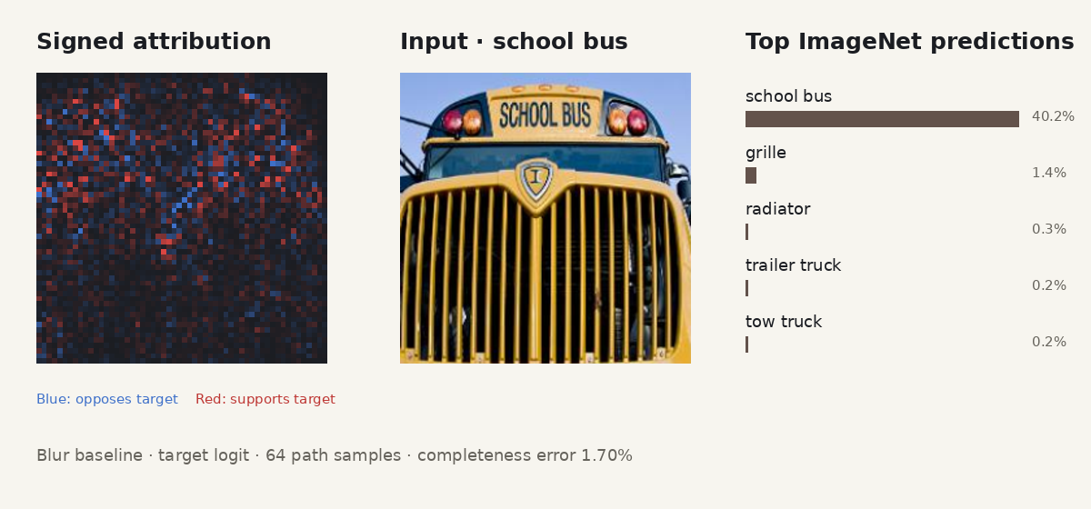
For the school-bus logit, 64 integration steps produce a 1.70% completeness error. The predicted class receives 40.2% probability, far above the next listed class, grille, at 1.4%. Attribution is concentrated around the front-facing geometry, lights, sign, and grille, with both supporting and opposing pixels. The dog and baboon examples need 256 steps to reach the same tolerance, illustrating why a fixed, low step count would give inconsistent numerical quality across inputs.

Text · how do tokens change sentiment?

The text experiment uses a DistilBERT classifier fine-tuned on SST-2 sentiment.^[04]04Sanh et al. (2019), “DistilBERT, a Distilled Version of BERT,” NeurIPS EMC² Workshop. Discrete token IDs cannot be interpolated meaningfully, so IG operates on the continuous input embeddings. Attribution is summed over each token’s embedding dimensions, leaving one signed value per token. Special tokens remain fixed and receive no displayed credit.

The controls cover six short linguistic patterns: positive wording, negation, contrast, intensification, mixed evidence, and punctuation. The baseline selector compares zero embeddings with the model’s [PAD] embedding. Hovering a token reveals its exact signed value; switching the output reveals whether a token supports the raw class score, the softmax probability, or the separation from the competing class.

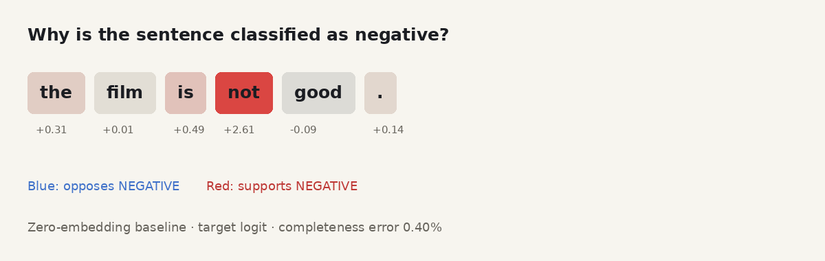
The default negation example is classified as negative. Against the zero-embedding baseline, not contributes $+2.609$ to the negative logit, while good contributes $-0.089$. In the contrast example, dull strongly supports the negative target and excellent opposes it. These values show that the classifier is not merely counting positive and negative words; the surrounding construction changes which class each token supports. They remain local explanations for the selected sentence and baseline, not reusable sentiment scores for those words.

Graphs · which atoms influence the molecular prediction?

The graph experiment moves the same calculation to molecular structure. A three-layer Graph Isomorphism Network (GIN) reads categorical atom features, passes messages along the bonds, pools the atom states, and predicts whether a molecule crosses the blood–brain barrier.^[05]05Xu et al. (2019), “How Powerful are Graph Neural Networks?” ICLR 2019. The BBBP dataset comes from MoleculeNet, a benchmark collection for molecular machine learning.^[06]06Wu et al. (2018), “MoleculeNet: A Benchmark for Molecular Machine Learning,” Chemical Science.

IG is applied after categorical atom features have been converted to continuous embeddings. The zero baseline removes the embedding signal; the training-mean baseline replaces every atom state with the average atom embedding from the training split. Node attributions are obtained by summing over embedding dimensions. Bonds remain visible to preserve molecular structure, but their line widths are not attributions.

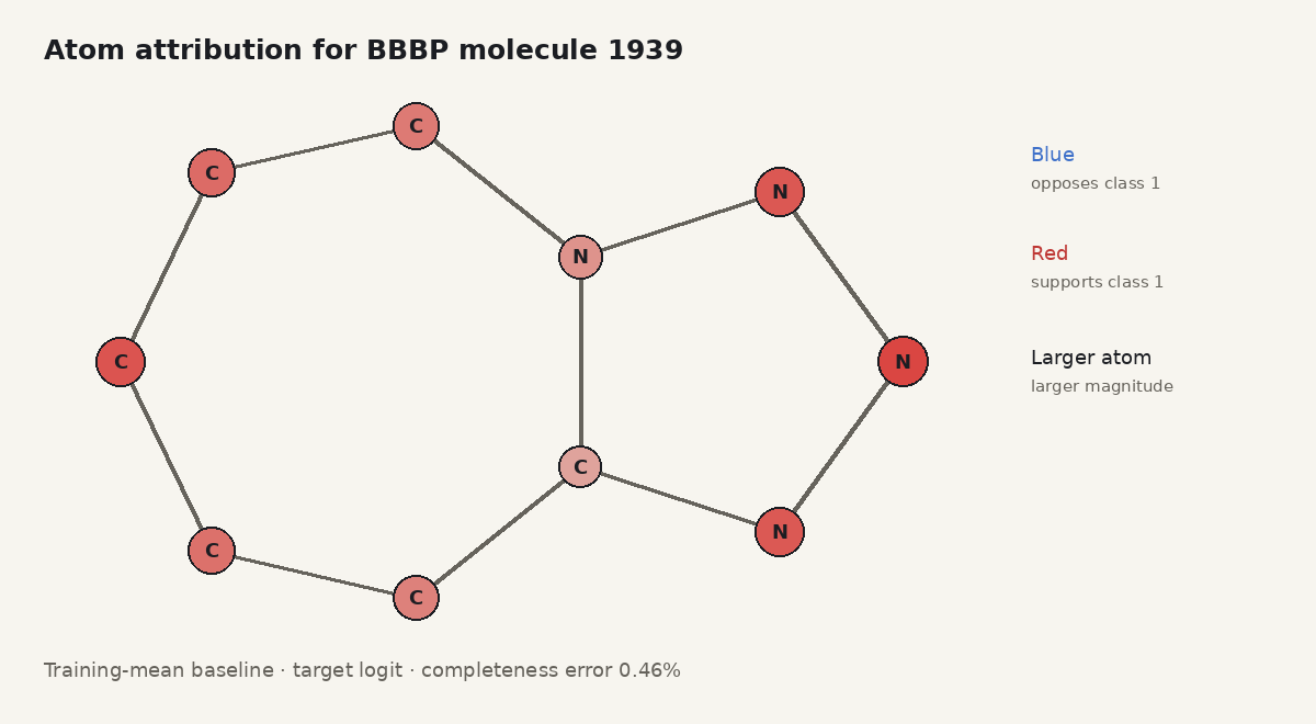
All eight displayed molecules, four from each true class, are classified correctly by the trained model. Larger, red atoms provide stronger support for the predicted class relative to the chosen baseline; larger, blue atoms oppose it. Comparing zero and mean baselines is especially useful here because an all-zero embedding is mathematically convenient but does not represent a chemically valid atom. The mean baseline asks the narrower question of how each observed atom state differs from an average training atom.

What transfers across modalities

The engine at the centre never learns what a feature is. Whether it faces a pixel, one dimension of a word embedding, or one dimension of an atom’s embedding, it asks for the same four things: a numeric input, a baseline of the same shape, a differentiable function that returns one score per point along the route, and a rule for collapsing raw feature dimensions into the unit shown on screen: a pixel, a token, an atom. Moving to a new modality means swapping those adapters, not the method.

What does not transfer for free is the meaning of absence. Blur keeps an image’s coarse content while erasing detail; a zero embedding and a [PAD] embedding stand for different kinds of missing word; a zero and a mean atom embedding are both artificial states a real molecule never occupies. The choice of output matters too: a probability can flatten in saturated regions, while a margin deliberately pits the top class against its closest rival. Completeness confirms the arithmetic adds up, but it cannot say whether the baseline or the output was the right question to ask.

Limitations

Integrated Gradients is local and non-causal. It explains a score difference along one chosen straight path, which may pass through inputs unlike the training distribution. Summing color channels, embedding dimensions, or atom dimensions also hides interactions inside each displayed unit. The examples are selected probes rather than a population-level audit, so they reveal model behavior without establishing global reliability.

Conclusion

The project connects attribution theory to a tested, modality-independent PyTorch implementation and deploys it on three real classifiers. Adaptive completeness checks prevent attractive but numerically weak maps from entering the public views. The resulting interfaces make baseline choice, output choice, and signed evidence inspectable rather than hiding them behind a single saliency image.