Course project · High-Level Computer Vision · Saarland University
From simulated roads to real-looking street scenes
How do pixel reconstruction, adversarial training, global attention, and a one-step diffusion prior change the translation from simulated to real driving images?
- Python
- PyTorch
- GANs
- Diffusion Models
The synthetic-to-real gap
Driving simulators can produce many camera frames together with labels for depth, objects, and road geometry. Real data are harder to collect and annotate. The pixels produced by a simulator, however, still have their own lighting, textures, and rendering style. A vision model trained only on those pixels may encounter a different image distribution when it reaches a real camera.
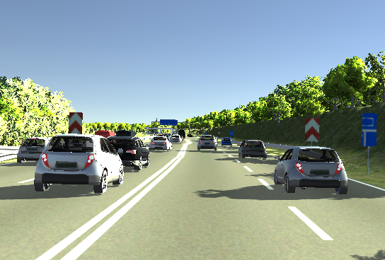
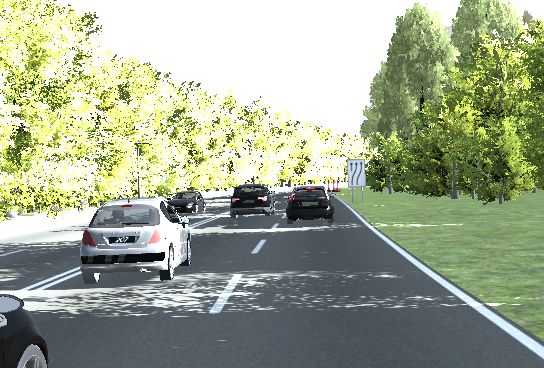
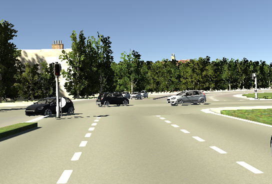
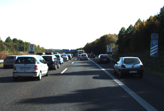
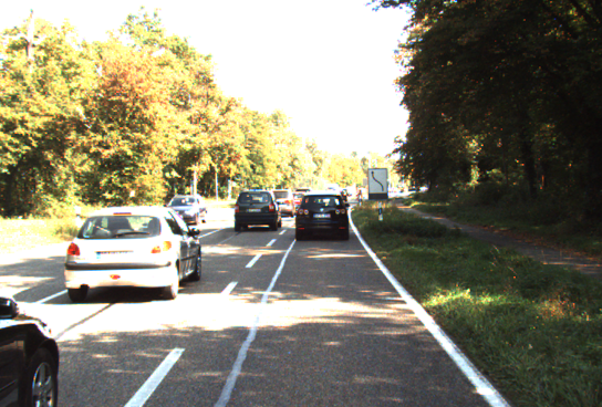
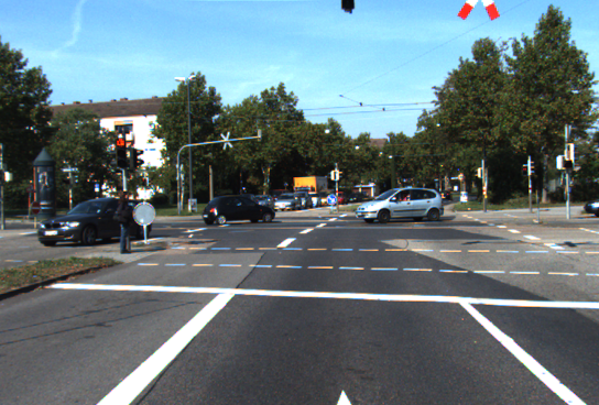
This project studied one narrow part of that problem: translate a simulated driving frame into an image with the appearance of a real street photograph while preserving the scene layout. The real images come from the KITTI benchmark, and the synthetic images come from Virtual KITTI, a virtual reconstruction derived from KITTI scenes.[01]01Geiger, Lenz, and Urtasun (2012), “Are We Ready for Autonomous Driving? The KITTI Vision Benchmark Suite,” CVPR 2012. [02]02Gaidon et al. (2016), “Virtual Worlds as Proxy for Multi-Object Tracking Analysis,” CVPR 2016.
The task resembles a controlled repainting. The road, cars, trees, and horizon should stay in place. Surface appearance should move from the synthetic domain toward the real domain. Unlike an ordinary color filter, the model has to learn that change from examples.
The project follows four stages: a reconstruction baseline, paired adversarial training, a transformer bottleneck, and a recent one-step diffusion backbone.
Preparing the data
The dataset is assembled by pairing each synthetic frame with the real frame that shares its filename, checking that both images open correctly, and noting which driving scene each pair belongs to. The result is a fixed list of 2,126 matched frames, split by scene:
- 1,554 training pairs from three scenes
- 233 validation pairs from a fourth scene
- 339 test pairs from a fifth scene, held out entirely
Splitting by scene is stricter than randomly splitting nearby video frames. Adjacent frames often show almost the same road from a slightly shifted camera position, so a random split could place near-duplicates in both training and validation. Holding out whole scenes instead asks the model to handle a location it has never seen.
All four methods receive RGB images resized to $256\times384$ pixels. The paired loader applies the same random horizontal flip to both images. CycleGAN-Turbo draws on the same frames but samples synthetic and real images independently, because its training does not need matched pairs.
Loading image comparison…
A · Synthetic
B · Synthetic
C · Synthetic
A · Real
B · Real
C · Real
Four ways to learn the translation
Each stage changes one part of the learning signal. Keeping the progression small makes the effect of each choice easier to inspect.
| Stage | Generator and training signal | Question asked |
|---|---|---|
| U-Net + L1 | Convolutional encoder-decoder with skip connections and pixel reconstruction only | Can a compact paired model learn the broad color and layout mapping? |
| Pix2Pix | The same U-Net plus a $70\times70$ PatchGAN discriminator | Does local adversarial feedback recover sharper texture? |
| Transformer + L1 | A parameter-matched U-Net with two transformer blocks at its bottleneck | Does global attention help without adversarial training? |
| CycleGAN-Turbo | A pretrained SD-Turbo generator adapted with LoRA and unpaired adversarial, cycle, identity, and LPIPS losses | Can a pretrained one-step image prior move appearance while retaining source structure? |
Stage 1 · a pixel baseline
U-Net was originally designed as an encoder-decoder with skip connections between matching resolutions.[03]03Ronneberger, Fischer, and Brox (2015), “U-Net: Convolutional Networks for Biomedical Image Segmentation.” The encoder compresses the image into increasingly abstract features. The decoder expands those features back to pixels. Skip connections let edges and spatial details bypass the narrow bottleneck.
The first model minimizes mean absolute pixel error:
\[ \mathcal{L}_{L1}(G) = \mathbb{E}_{x,y}\left[\lVert y-G(x)\rVert_1\right], \]where $x$ is a synthetic image, $y$ is its matched real image, and $G(x)$ is the generated image. L1 gives a direct and stable baseline. When several different real appearances are plausible for the same input, minimizing pixel error also encourages averaged colors and edges. That often appears as blur.
Stage 2 · asking a local critic
Pix2Pix adds a discriminator that sees the synthetic input beside either a real or generated image.[04]04Isola et al. (2017), “Image-to-Image Translation with Conditional Adversarial Networks,” CVPR 2017. Instead of judging the whole frame with one output, the $70\times70$ PatchGAN produces a grid of local real-or-generated decisions. The generator is trained with both signals:
\[ \begin{aligned} \min_G\max_D\;\mathcal{L}_{cGAN}(G,D) &\quad {}+ 100\,\mathcal{L}_{L1}(G). \end{aligned} \]The L1 term keeps the output near the paired target. The adversarial term rewards local patterns that resemble photographs, such as foliage, asphalt, and edge contrast. A patch critic can sharpen texture without needing to model an entire $256\times384$ image in one decision. It can also reward convincing local texture that is not globally clean.
Stage 3 · attention at the bottleneck
The transformer experiment keeps L1 as the only loss and replaces the U-Net bottleneck with two transformer encoder blocks. Self-attention lets a spatial position combine information from distant positions instead of relying only on a stack of local convolutions.[05]05Vaswani et al. (2017), “Attention Is All You Need,” NeurIPS 2017.
This is deliberately a small hybrid, not a full Vision Transformer. Its channel count was reduced to keep its parameter budget close to the convolutional U-Net. The comparison therefore asks whether long-range attention changes reconstruction under the same pixel objective, rather than combining attention with a new discriminator or loss.
Stage 4 · a one-step diffusion backbone
CycleGAN-Turbo adapts a pretrained SD-Turbo text-to-image model for image translation. The original method converts the diffusion pipeline into a one-step generator and trains small LoRA updates with adversarial and cycle-consistency objectives.[06]06Parmar et al. (2024), “One-Step Image Translation with Text-to-Image Models.” This experiment uses the prompts “a synthetic driving scene” and “a real photograph of a driving scene.”
Two mappings are trained. One moves synthetic images toward the real domain. The other maps real images back toward the synthetic domain. Passing through both should reconstruct the starting image:
\[ \begin{aligned} \mathcal{L}_{cycle} &= \lVert F(G(x))-x\rVert_1 \\ &\quad {}+ \lVert G(F(y))-y\rVert_1. \end{aligned} \]The actual training objective also includes perceptual cycle loss, identity loss, and vision-aided adversarial discriminators. This makes the final stage a hybrid: its generator comes from a pretrained one-step diffusion model, while adversarial and cycle losses adapt it without aligned pairs. Training ran for 5,000 optimizer steps and saved checkpoints every 500 steps.
Reading the evaluation
One number cannot describe image translation. The evaluator therefore measures four views of the same 233-frame validation scene. “Synthetic input” is the identity baseline: it sends the source image through unchanged.
L1 is the average absolute difference between paired pixels, while PSNR derives a reconstruction score from mean squared error. Lower L1 and higher PSNR indicate a closer pixel match. LPIPS compares deep visual features between paired images, with lower values indicating greater perceptual similarity.[07]07Zhang et al. (2018), “The Unreasonable Effectiveness of Deep Features as a Perceptual Metric,” CVPR 2018. KID compares the generated and real feature distributions rather than individual pairs, and lower is better.[08]08Bińkowski et al. (2018), “Demystifying MMD GANs,” ICLR 2018.
| Input or method | Checkpoint | L1 ↓ | PSNR ↑ | LPIPS ↓ | KID ↓ |
|---|---|---|---|---|---|
| Synthetic input | n/a | 0.2809 | 9.311 | 0.5670 | 0.2101 ± 0.0108 |
| U-Net + L1 | Epoch 3 | 0.1927 | 10.802 | 0.8062 | 0.5997 ± 0.0169 |
| Pix2Pix | Epoch 22 | 0.2054 | 10.323 | 0.5610 | 0.3538 ± 0.0109 |
| Transformer + L1 | Epoch 1 | 0.1783 | 11.317 | 0.8607 | 0.5148 ± 0.0152 |
| CycleGAN-Turbo | Step 5,000 | 0.2481 | 9.628 | 0.5120 | 0.1208 ± 0.0076 |
Results on the held-out validation scene. KID is reported as mean ± standard deviation across 100 random subsets.
The pixel metrics favor the transformer bottleneck, with U-Net and Pix2Pix in the next two positions. The perceptual and distribution views tell a different story. CycleGAN-Turbo is best on LPIPS and KID. Pix2Pix slightly improves on the unchanged synthetic input for LPIPS but remains farther away on KID.
That disagreement is expected from the objectives. The L1-only models are paid for matching a target pixel by pixel, so they learn smooth average structures when the pair is not perfectly aligned. Pix2Pix adds high-frequency detail, which helps perceptual similarity but also produces unstable local patterns. CycleGAN-Turbo does not chase the exact target pixels. Its pretrained image prior and unpaired losses instead change the source image toward the real-image distribution, which helps LPIPS and KID while giving up some L1 and PSNR.
The unchanged synthetic input has the second-lowest KID. This does not mean that no translation is needed. Virtual KITTI was built as a close virtual proxy for KITTI, so the two collections already share road-scene content. KID also measures distributions rather than whether one output matches its paired target.
Generated images
The image view keeps three validation examples fixed and changes only their generated columns. Select each architecture to compare the same synthetic inputs, generated outputs, and real references.
Loading image comparison…
A · Synthetic
A · Generated
A · Real
B · Synthetic
B · Generated
B · Real
C · Synthetic
C · Generated
C · Real
U-Net and the transformer preserve coarse road geometry but smooth away most texture. The transformer’s better paired pixel score therefore does not imply a sharper result. Pix2Pix restores edges and local contrast, but its patch-level feedback creates rippled and fragmented regions. CycleGAN-Turbo keeps the synthetic frame’s road, trees, and shadows recognizable while changing contrast and surface texture toward a camera image. It does not reproduce the real reference, which is consistent with unpaired training.
The two reconstruction models were also re-run several times; the best pixel model changed from run to run, while LPIPS stayed high for both. Pix2Pix and CycleGAN-Turbo were each evaluated once, so their ordering here is the outcome of this experiment rather than a general architecture ranking.
Limitations
The results use a modest 2,126-pair dataset at $256\times384$ resolution. Matching by filename gives related scenes, not exact pixel alignment, which limits what the pixel-based metrics can say. The same validation scene both selected the checkpoints and supplied this cross-method comparison, and the held-out test scene was not used for the figures here. Only the two reconstruction models were repeated across several runs; Pix2Pix and CycleGAN-Turbo were each evaluated once, under a single main configuration.
The evaluation covers pixel distance, perceptual features, and image-distribution distance. It does not include a human preference study or test whether a downstream detector trained on translated images performs better on KITTI. CycleGAN-Turbo also begins with a large pretrained image prior, whereas the first three generators are trained for this dataset from scratch, so the stages compare practical approaches rather than equal pretraining budgets.
Conclusion
The project forms one traceable line from raw driving frames to generated images. Holding out whole scenes keeps the model from being scored on places it has already seen; the pixel-only baselines show what a reconstruction loss does on its own; Pix2Pix shows what a local critic adds; the transformer isolates the effect of long-range attention; and CycleGAN-Turbo tests a recent pretrained diffusion generator that learns without matched pairs.
The main result is not a single winning score. Each objective leaves its own signature. Pixel reconstruction preserves the broad layout but averages away uncertain detail. Patch adversarial training adds texture and artifacts together. The diffusion backbone produces the most camera-like images under the perceptual and distribution metrics, while staying less faithful to the matched real pixels. That progression is the useful outcome: an end-to-end computer-vision experiment where the data choices, the training objective, the evaluation metric, and the generated image can all be read together.